Data Analysis Workflow – The Firehose

SOCI 3040 – Quantitative Research Methods

Class No.

04

Last Class or Next Class

  Reading Assignment

• Required: Ch 2
• Recommended: Ch 1

  Lecture Slides

In class work in RStudio! See notes below.

  Class / Lab Notes

1 Toronto Shelters – The Workflow Illustrated

Toronto has a large unhoused population. Freezing winters mean it is important there are enough places in shelters. In this example, we will make a table of shelter usage in 2021 to compare average use in each month. Our expectation is that there is greater usage in the colder months, for instance, December, compared with warmer months, for instance, July.

1.1 Import Libraries

You might see a lot of text print to the console when you import these libraries. You can ignore that for now!

library("janitor") # For cleaning and formatting column names and data.

Attaching package: 'janitor'

The following objects are masked from 'package:stats':

    chisq.test, fisher.test

library("knitr") # For creating tables and reports.
library("lubridate") # For working with dates and times.

Attaching package: 'lubridate'

The following objects are masked from 'package:base':

    date, intersect, setdiff, union

library("opendatatoronto") # For accessing Toronto's open data directly.
library("tidyverse") # A collection of R packages for data manipulation, visualization, and more.

── Attaching core tidyverse packages ──────────────────────── tidyverse 2.0.0 ──
✔ dplyr   1.1.4     ✔ readr   2.1.5
✔ forcats 1.0.0     ✔ stringr 1.5.1
✔ ggplot2 3.5.1     ✔ tibble  3.2.1
✔ purrr   1.0.2     ✔ tidyr   1.3.1

── Conflicts ────────────────────────────────────────── tidyverse_conflicts() ──
✖ dplyr::filter() masks stats::filter()
✖ dplyr::lag()    masks stats::lag()
ℹ Use the conflicted package (<http://conflicted.r-lib.org/>) to force all conflicts to become errors

library("here") # For managing file paths in a project-oriented workflow.

here() starts at /Users/johnmclevey/SOCI3040

The libraries listed here are essential for managing the workflow. Each library serves a specific purpose:

• janitor: Simplifies data cleaning tasks, such as renaming columns or identifying missing values.
• knitr: Provides functionality to integrate R code into reports and create professional tables.
• lubridate: Makes working with dates easier, such as extracting months or years from a date column.
• opendatatoronto: Offers tools to download and work with datasets provided by the City of Toronto.
• tidyverse: A suite of tools for data science, including dplyr for data manipulation and ggplot2 for visualization.
• here: Ensures consistent file paths regardless of the working directory.

1.2 Plan

The dataset we are interested in needs to have the date, the shelter, and the number of beds that were occupied that night. A quick sketch of a dataset that would work is shown in Figure Figure 1.

Figure 1: Quick sketch of a dataset

We aim to create a table summarizing the monthly average number of beds occupied each night. A sketch of such a table is shown in Figure Figure 2.

Figure 2: Quick sketch of a table

These sketches provide a conceptual understanding of the expected output and guide the workflow. First, we simulate data to refine our understanding of the data-generating process.

1.3 Simulate

Simulation is a crucial step for understanding the problem before analyzing real data. It allows us to:

1. Define assumptions about the data.
2. Create a test dataset that mimics the real dataset’s structure.

Here, we simulate a dataset representing the daily occupancy of three shelters over one year (2021):

set.seed(853)

simulated_occupancy_data <-
    tibble(
        date = rep(x = as.Date("2021-01-01") + c(0:364), times = 3),
        shelter = c(
            rep(x = "Shelter 1", times = 365),
            rep(x = "Shelter 2", times = 365),
            rep(x = "Shelter 3", times = 365)
        ),
        number_occupied =
            rpois(
                n = 365 * 3,
                lambda = 30
            )
    )

simulated_occupancy_data

# A tibble: 1,095 × 3
   date       shelter   number_occupied
   <date>     <chr>               <int>
 1 2021-01-01 Shelter 1              28
 2 2021-01-02 Shelter 1              29
 3 2021-01-03 Shelter 1              35
 4 2021-01-04 Shelter 1              25
 5 2021-01-05 Shelter 1              21
 6 2021-01-06 Shelter 1              30
 7 2021-01-07 Shelter 1              28
 8 2021-01-08 Shelter 1              31
 9 2021-01-09 Shelter 1              27
10 2021-01-10 Shelter 1              27
# ℹ 1,085 more rows

1.3.1 Code Breakdown:

1. set.seed(853): Ensures reproducibility of random numbers.
2. date column:
   • as.Date("2021-01-01"): Creates the starting date (January 1, 2021).
   • + c(0:364): Adds consecutive days to generate a sequence for the entire year.
   • rep(..., times = 3): Repeats the year-long sequence for three shelters.
3. shelter column:
   • Categorical variable indicating which shelter the data belongs to.
   • rep(..., times = 365): Repeats the shelter name for each day of the year.
4. number_occupied column:
   • Simulated using the Poisson distribution (rpois).
   • lambda = 30: Assumes an average of 30 beds occupied per shelter per day.

The simulated dataset has three columns:

• date: The date of observation.
• shelter: The shelter’s name.
• number_occupied: The number of beds occupied on that date.

1.4 Acquire

The next step is to download and process the real dataset from Toronto’s Open Data portal.

toronto_shelters <-
    list_package_resources("21c83b32-d5a8-4106-a54f-010dbe49f6f2") |>
    filter(name == "daily-shelter-overnight-service-occupancy-capacity-2021.csv") |>
    get_resource()

write_csv(
    x = toronto_shelters,
    file = here("data", "toronto_shelters.csv")
)

1.4.1 Code Breakdown:

1. list_package_resources():
   • Retrieves metadata for datasets in the specified package.
   • The package ID is specific to the Toronto shelter data.
2. filter():
   • Extracts the 2021 dataset by matching the dataset name.
3. get_resource():
   • Downloads the selected dataset.
4. write_csv():
   • Saves the dataset locally for future use.

Next, we clean the dataset:

toronto_shelters <-
    read_csv(
        here("data", "toronto_shelters.csv"),
        show_col_types = FALSE
    )

head(toronto_shelters)

# A tibble: 6 × 32
   X_id OCCUPANCY_DATE ORGANIZATION_ID ORGANIZATION_NAME        SHELTER_ID
  <dbl> <chr>                    <dbl> <chr>                         <dbl>
1     1 21-01-01                    24 COSTI Immigrant Services         40
2     2 21-01-01                    24 COSTI Immigrant Services         40
3     3 21-01-01                    24 COSTI Immigrant Services         40
4     4 21-01-01                    24 COSTI Immigrant Services         40
5     5 21-01-01                    24 COSTI Immigrant Services         40
6     6 21-01-01                    24 COSTI Immigrant Services         40
# ℹ 27 more variables: SHELTER_GROUP <chr>, LOCATION_ID <dbl>,
#   LOCATION_NAME <chr>, LOCATION_ADDRESS <chr>, LOCATION_POSTAL_CODE <chr>,
#   LOCATION_CITY <chr>, LOCATION_PROVINCE <chr>, PROGRAM_ID <dbl>,
#   PROGRAM_NAME <chr>, SECTOR <chr>, PROGRAM_MODEL <chr>,
#   OVERNIGHT_SERVICE_TYPE <chr>, PROGRAM_AREA <chr>, SERVICE_USER_COUNT <dbl>,
#   CAPACITY_TYPE <chr>, CAPACITY_ACTUAL_BED <dbl>, CAPACITY_FUNDING_BED <dbl>,
#   OCCUPIED_BEDS <dbl>, UNOCCUPIED_BEDS <dbl>, UNAVAILABLE_BEDS <dbl>, …

toronto_shelters_clean <-
    clean_names(toronto_shelters) |>
    mutate(occupancy_date = ymd(occupancy_date)) |>
    select(occupancy_date, occupied_beds)

head(toronto_shelters_clean)

# A tibble: 6 × 2
  occupancy_date occupied_beds
  <date>                 <dbl>
1 2021-01-01                NA
2 2021-01-01                NA
3 2021-01-01                NA
4 2021-01-01                NA
5 2021-01-01                NA
6 2021-01-01                 6

write_csv(
    x = toronto_shelters_clean,
    file = here("data", "cleaned_toronto_shelters.csv")
)

1.4.2 Code Breakdown:

1. read_csv(): Reads the downloaded CSV file.
2. clean_names(): Converts column names to snake_case for easier handling.
3. mutate(): Converts the occupancy_date column to a date format.
4. select(): Retains only the relevant columns (occupancy_date and occupied_beds).

1.5 Explore/Understand

The cleaned dataset is now ready for exploration. We compute the monthly average number of occupied beds:

toronto_shelters_clean <-
    read_csv(
        here("data", "cleaned_toronto_shelters.csv"),
        show_col_types = FALSE
    )

#| label: tbl-homelessoccupancyd-2
#| tbl-cap: "Shelter usage in Toronto in 2021"

toronto_shelters_clean |>
    mutate(occupancy_month = month(
        occupancy_date,
        label = TRUE,
        abbr = FALSE
    )) |>
    arrange(month(occupancy_date)) |>
    drop_na(occupied_beds) |>
    summarise(
        number_occupied = mean(occupied_beds),
        .by = occupancy_month
    ) |>
    kable()

occupancy_month	number_occupied
January	28.55708
February	27.73821
March	27.18521
April	26.31561
May	27.42596
June	28.88300
July	29.67137
August	30.83975
September	31.65405
October	32.32991
November	33.26980
December	33.52426

1.5.1 Code Breakdown:

1. mutate():
   • Adds a new column, occupancy_month, extracted from the occupancy_date.
   • Uses month() from lubridate to get the month name.
2. drop_na(): Removes rows with missing values in occupied_beds.
3. summarise(): Groups data by month and calculates the mean.
4. kable(): Creates a neatly formatted table.

The table provides insights into monthly shelter usage.

1.6 Share

The findings are summarized in a brief report:

“Toronto has a large unhoused population. Freezing winters mean it is critical there are enough places in shelters. We are interested to understand how usage of shelters changes in colder months, compared with warmer months.

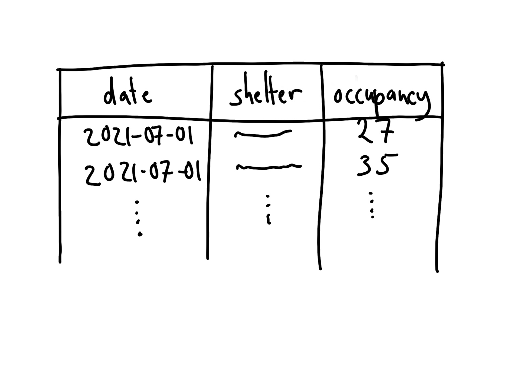
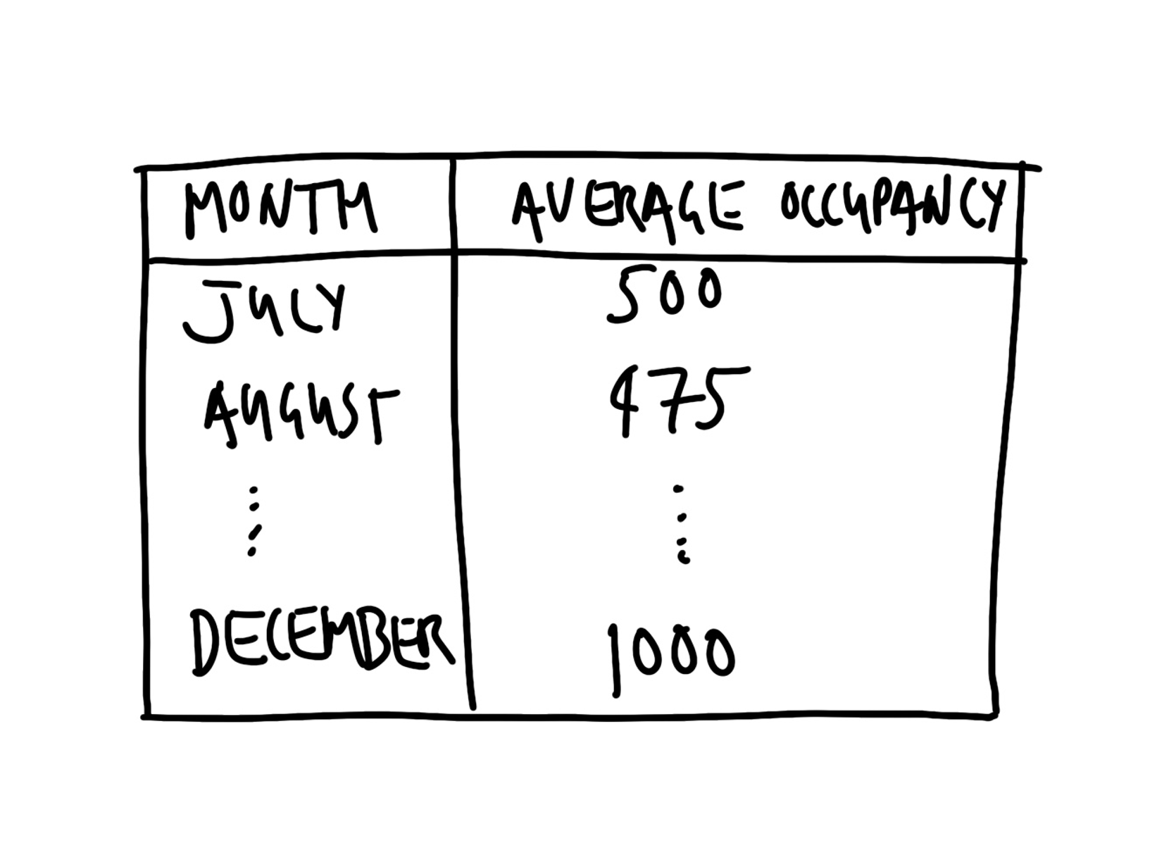
We use data provided by the City of Toronto about Toronto shelter bed occupancy. Specifically, at 4 a.m. each night a count is made of the occupied beds. We are interested in averaging this over the month. We cleaned, tidied, and analyzed the dataset using the statistical programming language R as well as the tidyverse, janitor, opendatatoronto, lubridate, and knitr. We then made a table of the average number of occupied beds each night for each month.

We found that the daily average number of occupied beds was higher in December 2021 than July 2021, with 34 occupied beds in December, compared with 30 in July. More generally, there was a steady increase in the daily average number of occupied beds between July and December, with a slight overall increase each month.”

1.7 SHARE!

Your turn…